
Having been self-quarantined at home now for several weeks I have a never-ending dream feeling of being on a train. Unfortunately, I am not the engineer of the train who sees where we are headed. I am at least half-way back in a train car that has very limited vision showing what is on the side and a little about where we have been. I have limited vision ahead to see where we are headed and where these tracks are taking us. As an actuary, I know how to project things into the future, but I am struggling to identify anyone who actually knows what the underlying assumptions should be. There are many models policymakers are relying on (e.g., The University of Washington model[1], The Cornell model[2], the Penn model[3], the UK model[4], etc.) but do any of these models reasonably predict where we are headed? I would hope so but the more I review them the less confidence I have about any of them. My need to know has encouraged some of my colleagues to help identify simple ways to validate what we are seeing, hearing and learning from the generally accepted models of today. This article will describe some of the things we believe to be critical in this process. It is the direct result of collaborating with a significant county here in California helping them answer this question.
Incidence and Emergence of COVID-19
Table 1 Starting Key Assumptions
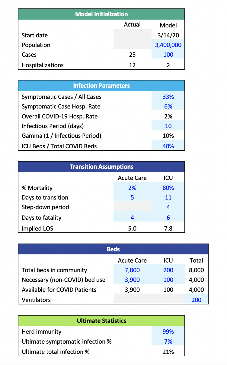
Table 1 summarizes a good way to get started. In addition to knowing how large the target population is when the first case is discovered, and the starting number of infections, the assumed growth rate or doubling rate is critical. The doubling rate is usually defined as the number of days it takes for the infected population to double in size. If the doubling rate assumption is 4 days and today there are 100 cases, our model would project that four days from now there would be 200 cases. One of our most recent projections started with a doubling rate of 3.5 and increased that to slightly more than 7.0 as the result of multiple interventions in this market. Those doubling rates were consistent with growth rates of 22% decreasing to about 10%. For this particular region, this assumption had an excellent fit with the emergence of data to date. However, it is imperative to point out that the doubling rate assumption is not static. It will vary as time progresses and the model population either reduces virus transmissibility through interventions like increased handwashing or mask-wearing or increases transmissibility by, say, frequently gathering in large groups. As the virus’s transmissibility increases, the doubling rate decreases. As transmissibility decreases, the doubling rate increases. Below, I’ll discuss how to incorporate this dynamic assumption into the model.
The impact of different doubling rate or growth rate assumptions is significant. In modeler-speak, the output is very sensitive to this variable. This is not an assumption to be taken lightly. For example, a seemingly minor shift in this assumption can change the time required to infect the entire population by 20 days.
The larger the number of initial cases, the faster the spread of the infection across the population. In light of under-reporting, inadequate initial testing, and a general lack of information when COVID-19 emerged, an initial assumption of multiple cases may be reasonable. As shown in Table 1, we initialized our model at 20 cases rather than one, because the folks on the ground trusted the data from that time on much more than the initial data. Given a lack of confidence in the initial data, we focused on calibrating our model to the more recent counts as well as the emerging trends. Given the rapid developments of interventions that would affect the doubling rate, the modeler must be careful not to overfit the data. Initial data, even if representative of a statistically valid sample of the population, might have an inherent doubling rate substantially different than the current doubling rate. The modeler should be aware that there may be multiple inflection points in the growth curve and adjust projections accordingly.
The infection rate for the population helps to set an initial boundary point to determine what will the likely outcome be. For our model, we did not allow the infection rate to flow through the results because we have so little confidence about the range of appropriate values for it. In other words: no one knows today what the ultimate infection rate will be. Instead, we tested the implications of some sample infection rates to use as reasonability checks for the model output in our validation process. Testing this assumption can help understand the timelines of the growth in infections.
Interventions are important today. In our community we limited the size of gatherings, quickly shifting to closing down restaurants/bars, schools and any business that was viewed as not necessary. Work/stay at home became the norm and just this week, masks outside of one’s home became mandatory. These are a series of interventions each hoping to extend the doubling rate from its initial level. Our modeling approach handles as many interventions as are applied in a community.
Figure 2 shows growth in COVID-19 cases under three scenarios: no intervention, one moderate-impact intervention, and two moderate-impact interventions. Under the “No intervention” scenario, 95% of the population is infected by the end of May. The rapid spread clearly demonstrates the impact of the doubling rate assumption (i.e., 3.5 days in this scenario).
Fortunately, we do have interventions within our grasp to slow the spread of this infection. Many local and state governments deployed some of these in the past few weeks. Figure 2 demonstrates the more moderate growth in COVID-19 cases given the interventions. The “Intervention 1” scenario demonstrates the impact of the doubling rate increasing from 3.5 to 5 days over a 10-day period. The “Intervention 2” scenario includes the 3.5-to-5-day intervention, as well as a subsequent intervention which increases the doubling rate from 5 days to 8 days over a 10-day period.
Figure 2 Emergence of COVID-19 Cases Under Multiple Scenarios
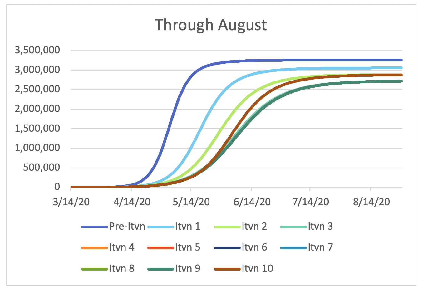
By the end of April, there is a 96% reduction in the case count under the “Intervention 2” scenario relative to the “No Intervention” scenario.
Figure 2 clearly shows the impact of the assumed interventions on the growth in cases. This is what has been talked about as bending or flattening the curve.
Impact on Hospital Supply
In this market, there are about 8,000 licensed beds of which in recent times less than 5,000 have been staffed. Estimates are that up to 4,000 are occupied by patients that can’t be moved elsewhere or eliminated. The major health planning concern is when will we run out of beds to take care of the surge from COVID-19.
The unfortunate result of a projection reflecting the intervention announced 3/19/2020 (as modeled in the “Intervention 1” scenario above) estimates that the peak of hospital resources will occur late May 2020 with a needed bed count of almost 300% of capacity. As discussed above, this scenario assumes that the initial intervention extended the doubling rate from 3.5 days to 5.0 days (decrease in growth rate from 22% to 15%). A logical follow-up question is what doubling rate reduces the demand to match the resources we have available. A doubling rate of 12.0 days lowers the needed beds to 8,000, but this doesn’t consider others who also need the beds. It takes a doubling rate of at least 16.0 days to get the demand below 4,000 beds.
The above shows the result of significant changes in doubling rates. But what intervention(s) can achieve these results? Literature suggests a wide extreme between interventions:
- Full lock-down (Ebola method): forced program so the disease can’t spread, short epidemiologic curve and fewer cases
- Slow the spread (Flu method): virus doesn’t go extinct, becomes another endemic virus which gets spread with less potency
The Ebola method requires the ability to truly shut down society (unlikely in the US) and you prevent the introduction from another source (i.e., travel from outside the US). The Flu method is the less preferred approach but recognizes the difficulty of shutting down society.
Several other initiatives have now been implemented (i.e., masks, law enforcement, etc.). This results in a delayed peak demand until the first week of June. The major challenge for our public health experts is how do we significantly impact the doubling rate using methods we have a reasonable chance of implementing. What haven’t we done that we can do? The outlook is grim unless we get very creative. The development of a vaccine would be beneficial, but it is not a viable option in the short term (i.e., before the early June surge in our currently modeled scenario).
Summary
Back to my train ride. Perhaps it is good I can’t see ahead. I don’t want to see the damaged bridge over the canyon ahead. I just hope the repair team can fix it before we arrive in the coming weeks.
Endnotes
[1] https://covid19.healthdata.org/projections
[2] https://hpr.weill.cornell.edu/cornell-covid-caseload-calculator-c5v
[4] https://www.imperial.ac.uk/mrc-global-infectious-disease-analysis/covid-19/
About the Author

About the Author

Any views or opinions presented in this article are solely those of the author and do not necessarily represent those of the company. AHP accepts no liability for the content of this article, or for the consequences of any actions taken on the basis of the information provided unless that information is subsequently confirmed in writing.