Medical IBNR; Traditional Approach with a New Twist

Medical claims reserving has remained relatively unchanged for decades. The traditional approach to calculating IBNR reserves, that will be defined later in this article, has stayed the same even though technology and computing power has improved exponentially over the previous decades. According to Dr. Michio Kaku, a theoretical physicist and futurist, “Today, your cell phone has more computer power than all of NASA in 1969, when it placed two astronauts on the moon”. Should our reserving methods have changed with all the technological enhancements, or did early actuaries have the method right?

This article will offer a new twist on a classic method of IBNR estimation, while keeping the calculations outside the “black boxes” that are so prevalent today. This article will also offer some ideas to help improve the power of your IBNR model by looking at:

• What completion factor averaging method is best
• What data elements really should be reviewed
• What are the key traps in IBNR?
• What level of detail should you do your IBNR estimates (how many different cells)?
• What else can an IBNR model be used for?

Actuarial work is very data driven and what would it look like if we got away from looking at numbers and started looking at pictures and graphs in order to help make better estimates. This article will also explore some data visualization approaches and how they can revolutionize the IBNR estimation process.

The Traditional IBNR Approach

The traditional IBNR reserving approach uses claims lag triangle information to estimate completion factors (i.e., payment patterns) to then estimate ultimate incurred claims and the estimated outstanding liability. The key to good IBNR estimates under the traditional approach is the calculation of the most recent incurred month’s liabilities where most of the IBNR is found. These months have the least amount of data, and include the most actuarial judgement and often involve manual overrides to the traditional developmental approach.

Completion factor averaging

Completion factors are the key to any good IBNR model using the traditional method. There are many different ways that completion factors can be derived, but the question often comes down to “what method of averaging actual completion factors should I use”. There are three frequent types of averaging we see in our review of IBNR models:

• Simple Averages: 3-month, 6-month, or 12-month
  • Average of the most recent 3, 6, or 12 actual completion factors
• Smoothed Averages 6 of 8, or 10 of 12
  • Throw out the high and the low and then average the remaining completion factors
• Harmonic Averages
  • take the reciprocal of the average of reciprocals of the completion factors for various time periods.

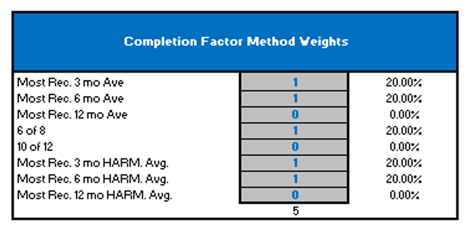
All of these methods may work reasonably well at various points in time and under certain scenarios. Instead of picking the one that you think might be the “best” all the time, wouldn’t it be better to take a weighted average of the various methods and determine an average completion factor (i.e., essentially an average of averages). It is my opinion that in a best in class IBNR model you should be able to average multiple methods. Another nice byproduct of being able to average different methods is that it also opens up the opportunity to easily run scenarios of the methods. By changing the weighting or just selecting different methods, you can test different scenarios. Below is an excerpt out of the AHP Claims Projection SystemTM that allows for averaging and or simulating different methods of completion factor weighting.

In reality, the actuary will override these completion factors for the most recent months based upon unique patterns of claim payment observed at the time of calculation, but it is still important to get a reasonable first pass.

Required Data Elements

In order to calculate IBNR estimates there are only two required elements that most models need in order establish an estimate and they are, members and claims. Claim triangles come in different shapes, sizes, and orientation. I prefer columns of individual paid months and rows of incurred months, but as long as the data has both elements it does not matter.

Including a few additional data elements in the IBNR model can provide very useful and helpful information. With the passage of ACA and the increased attention to loss ratios, by including premium in your IBNR model you will be able to make real time estimates of medical loss ratios. This can provide an early warning sign of experience deterioration.

Most IBNR estimation models can make reasonable estimates by following the basic developmental approach to estimation, but an amazingly IBNR models are set up in a way to clearly show how adequate your historical estimates have been using the most recent runout. This includes restatement of prior liabilities and also analysis to show what type of provision for Adverse Deviation (i.e., PAD) should be made. Per the Actuarial Standards of Practice (ASOP 5) on IBNR estimation it is important to make a best estimate and add a Provision for Adverse Deviation (PAD). Many actuaries use “rules of thumb” when setting and including estimates of PAD. Even with very limited effort it is possible to develop updates of PAD requirements each month based upon actual claim payment history using statistical analysis. In addition there are many other data elements that could be included in a best in class IBNR tool including: special adjustment for Large or shock Claims, Utilization rates, Seasonality analysis, and Loss Ratio analysis.

Key Traps in IBNR Estimation

There are many traps that actuaries fall into when doing IBNR. One of the main traps that we have seen many times is that actuaries try to take simple math and make it more complex. As talked about earlier in this article the basic developmental method for calculation IBNR is not very complex and has been around for a long time. Over time many actuaries have taken the basic math and tried to expand on it in order to make it more complex. It might be adding a complex multivariate regression or simulating obscure assumptions, but most of the time these findings are not presented in the output and have very little effect on the outcomes. Medical IBNR does not require sophisticated mathematics, but rather good actuarial judgement. Many times IBNR estimates that cannot be explained very simply to a stakeholder are not worth the sophistication used in refining the estimation process.

The second trap that many actuaries doing IBNR fall into is that they often set predetermined expectations of what the IBNR amount should be. These may be the result of past estimates that they or other actuaries made, or it may be from expectations that may have been communicated by other interested parties. Each month the IBNR estimate needs to be calculated independently without any predetermined bias. It is hard to completely eliminate bias, but estimates need to reflect the data used to make the estimate without bias. With that being said, monitoring previous estimates needs to be part of any best in class IBNR process. If you do not know how adequate or inadequate past estimates have been, how do you plan to be able to make more reasonable estimates in the future.

Third trap that many people fall into is that seasonality is only an output of the IBNR model and not a determining factor in setting IBNR. Seasonality is about as important to IBNR estimation as any type of metric. It is my opinion that it is close to impossible to set IBNR estimates without reviewing the seasonality. Seasonality is very present in medical claims and should be reviewed as to not overstate or understate IBNR liabilities.

The fourth and final trap to be discussed in this paper is the trap that “the IBNR model is always right”. There are no known perfect IBNR models, and there is no perfect IBNR estimation process that can be used without human intervention or actuarial judgement. Too often the prevailing view is that the IBNR model does 90% of the work and the user does only 10%., This is unreasonable since actuarial judgement is so critical to good estimates. It is my opinion that the computer should do only about 10% of the work and the actuary should review and adjust spending most of the time refining the estimates. Complete and extensive monitoring reports are key to the iterative process of reviewing and refining IBNR estimates.

What level of detail should you reflect in your IBNR estimates?

Users often ask this question when setting IBNR for subsets of the company’s business (i.e., lines of business). We once had a client that calculated their IBNR liabilities by making individual estimates at over 450 different splits (cells). Some cells ranged from having 50,000+ members while other had less than 10 members. The client’s rational for having so many different cells was that this was the level of detail that the IBNR was needed in order to put it into the general ledger and other detailed financial reports. At this organization they had a team of 10 plus people spending many days calculating all of the 450 IBNR estimates. In one of our meetings we asked them if they had every thought of doing an allocation instead of doing individual estimates. Their answer was that they would rather use more FTE’s and get better answers than do an allocation in order to get the estimate into the general ledger more efficiently.

So what level of detail is right? I do not believe that there is a magical number of cells that is the “right” answer all the time, but I do know that doing individual estimates does not always create the most reasonable answers as the client above thought. In order to calculate a reasonable estimate there needs to be a large enough number of people in each cell to reduce the volatility and create more stable patterns. Doing IBNR on 10 people holds no purpose and it is my professional opinion that making estimates on a population less than 2500 people is often too noisy to make reasonably consistent estimates.

When the consulting arrangement was completed the client above started calculating on about 45 cells, only about 10% of the amount previously calculated. We recommended that number being between 12 and 20, but was believed that the 45 could still be done while maintaining actuarially sound principles. This change did produce a bit of an IBNR change, as they went from being what they thought was adequately reserved, to being far under reserved and in need of major restatements. They blamed this change on the model and did not understand that the way they were using the model in the past did not fully utilize the power of the model and thus did not produce reasonable estimates. This is often called the “GIGO affect”, meaning garbage in garbage out. You cannot put data into a model that is incomplete and deficient and hope to get good estimates out the other side.

Estimates should be made at a level that ensures each cell has adequate membership and history in order to understand historical patterns and thus project appropriate claim liabilities. There sometimes are reasons to split the data by plan (benefit design), area (geographic), Line of business (Commercial, Medicare, Medicaid), or place of service (Inpatient vs. Outpatient), but it is not always needed. The larger the population, the more cells that can be justified.

What else can an IBNR model be used for?

IBNR models should be used for more than just calculating IBNR. If IBNR is all the user is concerned about, they need to take a step back and see what else could be looked at while doing the IBNR. IBNR models should be used as an early warning sign to what is going on in the company as a whole or in a specific line of business. If the estimated incurred claims are going through the roof it might be time to look at the pricing and or benefit designs to see about a change that needs to be made.

Loss Ratios have become very popular especially with the passage of ACA. By simply inputting premium into an IBNR process the user should be able to get an up to date estimate of what the basic medical loss ratio is. This is not a full ACA loss ratio including other elements, but it gives an early warning sign to a potential problem in the pricing.

Claim seasonality is an output of a good IBNR model and should be viewed as often as looking at the IBNR. Many companies spend countless hours creating advanced seasonality models, when most of the data is already easily available in a good IBNR model. Every month claim information is loaded into the model by paid and incurred months and would be easy to review seasonality at the same time.

Utilization can often affect IBNR dramatically, and for this reason reviewing utilization is a good way to monitor what is going on in the business. It might be monitoring admits for an Inpatient IBNR cell, or specialty scripts for an RX IBNR. Finding simple metrics to look at can often help unlock some of the mystery of the changing IBNR.

Data Visualization

So much of actuarial work is about looking at numbers and calculating factors. What would happen if for a moment we went away from trying to find a more complex equation with more variables and tried to find more simple ways of looking at factors, numbers, and outcomes. How would IBNR estimation change if we looked at more graphs and visuals and less decimal points. The numbers and calculations are of utmost importance, but finding better ways to look at them is the best way to change IBNR in the future. The developmental approach to IBNR estimation has worked for decades and it is the job of the actuary to find better ways to show it.

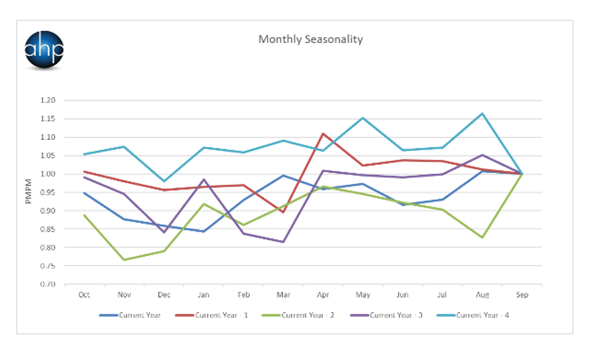
Below are some examples of graphs that could be used instead of looking just at the raw numbers. The Graph-1 shows seasonality by year. The graph shows 5 years of data and all are calibrated to the same starting month of the year. You can easily see the patterns over time.

Graph 1

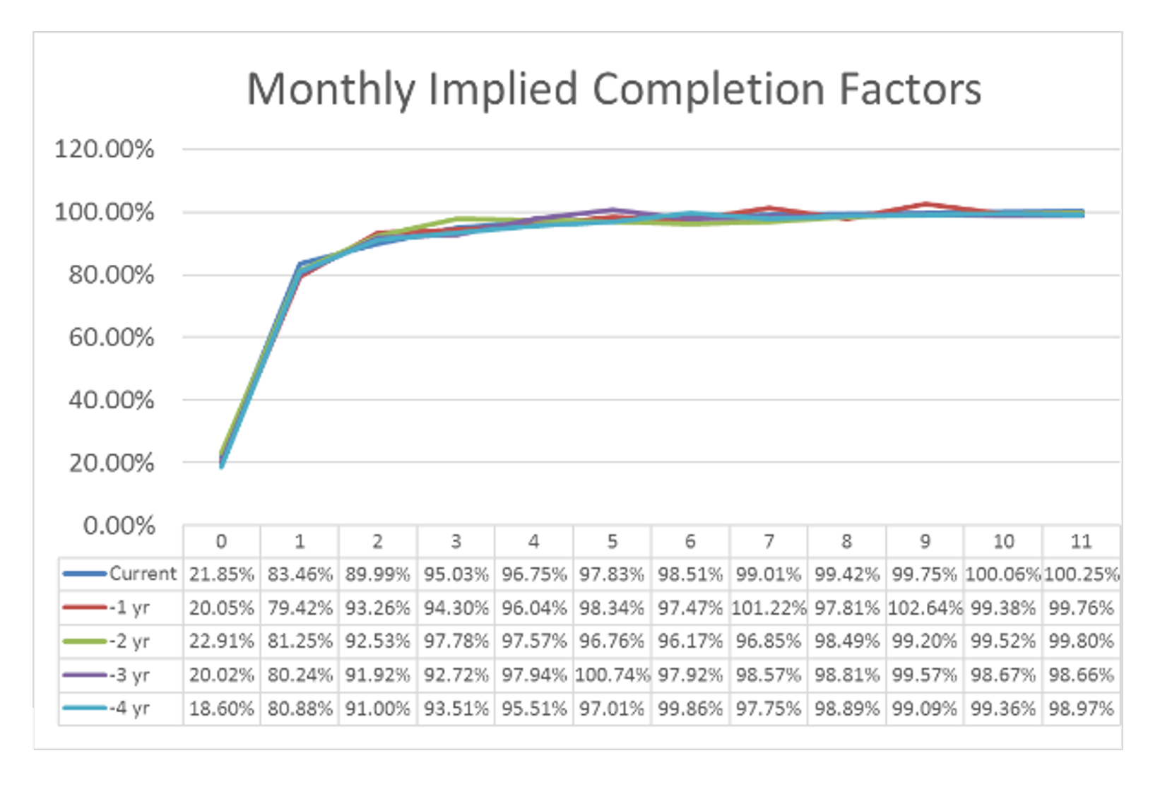
Graph 2 shows the implied completion factors. As is common in IBNR estimation there are manual overrides done by the user. This graph quickly shows if the manual estimates made make the completion factors look drastically different than the previous years.

Graph 2

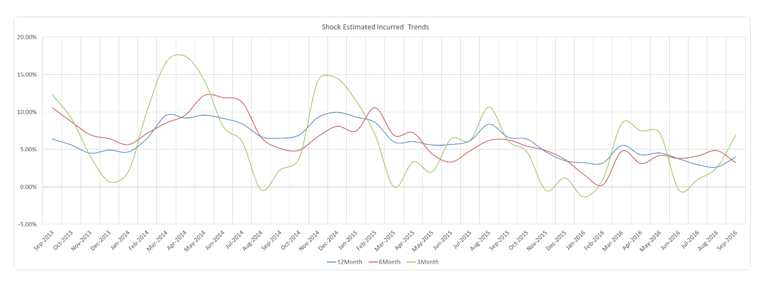
Graph 3 shows the monthly estimated incurred claims trends. This graph clearly shows the cyclical patterns found in claim activity. This graph is also able to show the difference in the 3, 6, and 12 month trends. Each of these trends holds a different purpose and seeing them together gives a great picture of what is going on with the trends.

Graph 3

Summary

The math behind medical claims reserving / IBNR reserving have remained relatively unchanged for decades. As we step into the future, the methods do not need to change but rather the way we look at them needs a bit of a paradigm switch. IBNR no longer should be an estimate that is only used to fill a line on the general ledger but rather it should be used to assess the overall health of a company through monitoring reports in the model. Models do not need to get more complex, but rather need to be more simplified using more visuals in order to get to a reasonable answer. Instead of increasing the complexity of the formulas used we should work toward automating manual tasks in order to spend more time actually trying to understand what is going on in the data and how it needs to be adjusted. As long as there are actuaries, there are going to be spreadsheets with countless lines of numbers. As we move forward with IBNR estimation the top priority needs to be maximizing the power and usefulness of the model, while making the output easy to understand and implement by non-actuaries. In the end, an estimate is only a number to a person that cannot understand what it is based on.